Tutorial
This page walks through a complete gFlex workflow using a physically motivated 2-D scenario: a circular surface load on a plate whose elastic thickness \(T_e\) varies smoothly from west to east. The same scenario underlies the gFlex logo.
The workflow covers:
setting up the grid, material parameters, variable \(T_e\), and load;
running the 2-D finite-difference solver;
visualising results with the built-in matplotlib plots; and
exporting to Blender for a publication-quality 3-D render.
Physical scenario
A circular volcanic edifice sits at the centre of a 750 × 750 km domain. The lithosphere beneath it is laterally heterogeneous: \(T_e\) rises from 15 km in the west to 35 km in the east across a sigmoid transition. Thinner lithosphere deflects more sharply and over a shorter wavelength; thicker lithosphere spreads the load farther and produces a more prominent forebulge.
The contrast is visible in the result: the depression is asymmetric — deeper and more confined on the soft (west) side, broader and shallower with a clearer forebulge on the stiff (east) side.
Grid and material parameters
import numpy as np
from gflex import F2D

# Grid: 150 × 150 cells at 5 km → 750 km domain
nrows = ncols = 150
dx = dy = 5000.0  # m

# Physical parameters
E        = 65e9    # Pa  — Young's modulus
nu       = 0.25   # —   — Poisson's ratio
rho_m    = 3300.0  # kg m⁻³ — mantle density
rho_fill = 0.0    # kg m⁻³ — infill density (air)
g        = 9.8    # m s⁻²

# Cell-centre coordinate arrays
xi = (np.arange(ncols) + 0.5) * dx
yi = (np.arange(nrows) + 0.5) * dy
XX, YY = np.meshgrid(xi, yi)
cx = cy = 0.5 * nrows * dx   # domain centre
Variable elastic thickness
A sigmoid transition from \(T_e = 15\) km (west) to \(T_e = 35\) km (east) over a characteristic length of \(8\,\Delta x = 40\) km:
Te_min, Te_max = 15e3, 35e3          # m
x_norm  = (XX - cx) / (8 * dx)      # normalised distance from centre
Te_grid = Te_min + (Te_max - Te_min) * 0.5 * (1.0 + np.tanh(x_norm))
Circular load
The load radius is set to \(1.5\alpha\), where \(\alpha\) is the flexural parameter computed from the mean \(T_e\):
Te_mean  = Te_grid.mean()
D_mean   = E * Te_mean**3 / (12.0 * (1.0 - nu**2))
alpha    = (D_mean / ((rho_m - rho_fill) * g))**0.25

load_radius = 1.5 * alpha
R  = np.sqrt((XX - cx)**2 + (YY - cy)**2)
qs = np.where(R <= load_radius, 3e7, 0.0)   # 30 MPa inside, 0 outside
A 30 MPa load over a ~60 km-radius circle is equivalent to roughly 930 m of mantle-density rock — comparable to a large volcanic plateau or the distal part of a sedimentary basin.
Running gFlex
flex = F2D()
flex.quiet = True

flex.method  = 'fd'

flex.g        = g;     flex.E  = E;    flex.nu = nu
flex.rho_m    = rho_m; flex.rho_fill = rho_fill
flex.T_e      = Te_grid
flex.qs       = qs
flex.dx       = dx;    flex.dy = dy

flex.bc_west = flex.bc_east = flex.bc_south = flex.bc_north = 'zero_moment_zero_shear'

flex.initialize()
flex.run()

w = flex.w   # deflection array [m]; negative = downward
# flex.output() here to save/plot via the built-in helpers.
# flex.finalize() when you are done with w and qs (frees all state).
The result: ~54 m of central subsidence and ~1 m of forebulge uplift. The asymmetry between the west (soft) and east (stiff) sides is clear in the output.
Matplotlib visualisation
The built-in Plotting() method produces a figure for whatever outputs
are available. For a 2-D run, call twoSurfplots() directly; when
Te is a 2-D array it shows three panels (load, elastic thickness,
deflection):
import matplotlib.pyplot as plt

flex.twoSurfplots()   # load, Te, and deflection (three panels for 2-D Te)
plt.show()
Or, for the three-panel view used in this example (load, \(T_e\),
deflection side by side), plot the arrays directly. This requires the
cmcrameri colormap package (pip install 'gflex[plot]'):
from cmcrameri import cm as cmc

w_abs = float(np.abs(flex.w).max())

fig, axes = plt.subplots(1, 3, figsize=(14, 4.5))

axes[0].imshow(flex.qs / (rho_m * g),
    extent=(0, dx/1000*ncols, dy/1000*nrows, 0),
    cmap=cmc.lajolla_r, aspect='equal')
axes[0].set_title("Load thickness, mantle equivalent [m]")

axes[1].imshow(flex.T_e / 1e3,
    extent=(0, dx/1000*ncols, dy/1000*nrows, 0),
    cmap=cmc.roma, aspect='equal')
axes[1].set_title(r"Elastic thickness $T_e$ [km]")

axes[2].imshow(flex.w,
    extent=(0, dx/1000*ncols, dy/1000*nrows, 0),
    cmap=cmc.vik, vmin=-w_abs, vmax=w_abs, aspect='equal')
axes[2].set_title(r"Deflection $w$ [m]")

for ax in axes:
    ax.set_xlabel("x [km]"); ax.set_ylabel("y [km]")
plt.tight_layout(); plt.show()
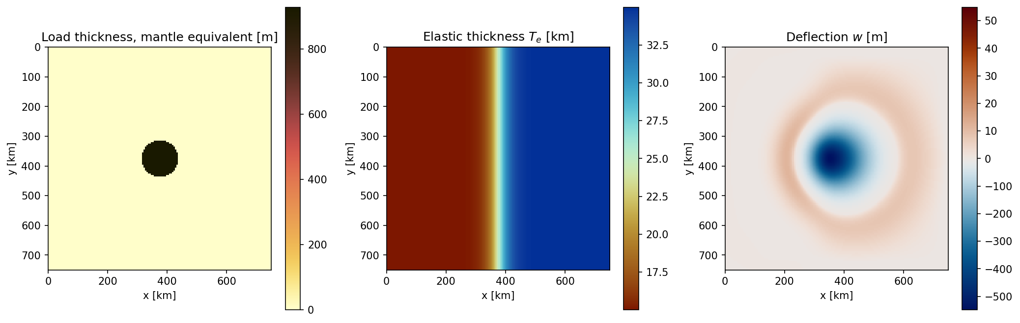
Left: circular load (dark = heavier; lajolla_r colormap). Centre: sigmoid \(T_e\) transition from 15 km (west, warm red) to 35 km (east, cool blue-green); roma colormap. Right: deflection coloured with the vik diverging colormap (blue = subsidence, red = uplift); the asymmetry between soft and stiff sides is clearly visible.
3-D render with Blender
gflex.export_for_blender() converts the deflection array into a
pure-Python mesh file that Blender’s embedded interpreter can read without
NumPy or gFlex installed:
from gflex import export_for_blender

export_for_blender(
    flex.w, flex.dx,
    path='/tmp/gflex_blender_mesh.py',
    z_exaggeration=200.0,
    qs=flex.qs,
    Te=flex.T_e,
    rho_m=rho_m,
    g=g,
)
Then render headless with the companion scene script:
blender --background --python docs/examples/blender_flexure.py
The script reads /tmp/gflex_blender_mesh.py by default (edit the
MESH_FILE constant at the top to change the path) and writes a PNG with a
transparent background, ready to composite into a paper or presentation.
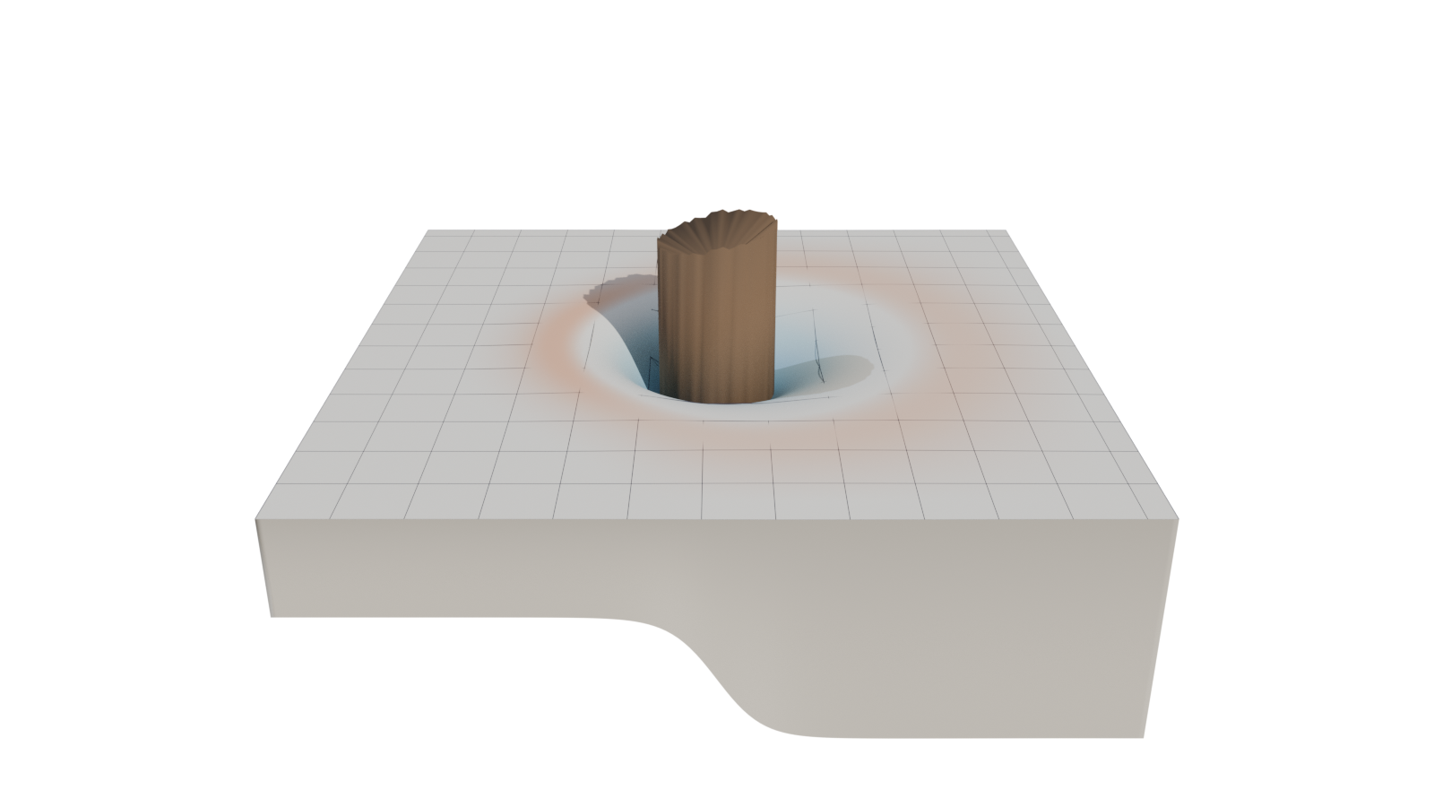
Blender render of the same scenario: vik-coloured deflection surface, wireframe \(T_e\) grid, \(T_e\) floor slab, and dark basalt load cylinder whose base deforms with the plate. Vertical exaggeration is 200×; the domain is 750 × 750 km.
Note
The scripts in docs/logo/ reproduce this scenario at the settings used
for the gFlex logo (generate_logo_data.py, blender_logo.py,
add_logo_text.py, make_logo.sh). They differ from
docs/examples/blender_flexure.py in camera framing, load representation,
and text overlay — tuned for logo aesthetics rather than scientific figure
production.