Boundary Conditions

Boundary conditions specify what happens at the edges of the modelled domain. gFlex supports six named conditions for the finite-difference (FD) solver; four impose constraints on which plate mechanical quantities — deflection, slope, bending moment, and shear force — vanish at that edge; one (periodic) connects opposite edges in a wrap-around domain; and one (no_outside_loads) automatically extends the domain before solving. Five short aliases (clamped, pinned, free, mirror, infinite) are also accepted. The interior finite-difference stencils are derived in Theory and Numerics; this page covers the boundary-node stencils and their physical interpretations.

For the spectral (FFT) solver, boundary conditions are handled per opposite-edge pair (W/E and N/S independently): if both sides of a pair are set to periodic, that axis uses an exact periodic solution; otherwise the axis is zero-padded by \(\approx 4\alpha\) before solving, which is equivalent to no_outside_loads for that axis. The analytical-superposition (SAS / SAS_NG) methods always assume no_outside_loads.

Overview of all boundary conditions and their applicability across solver families (FD, FFT, SAS) and dimensionality (F1D, F2D).

The following figure from Wickert (2016) illustrates four of the five mechanically-named conditions (zero_displacement_zero_moment was added after publication):

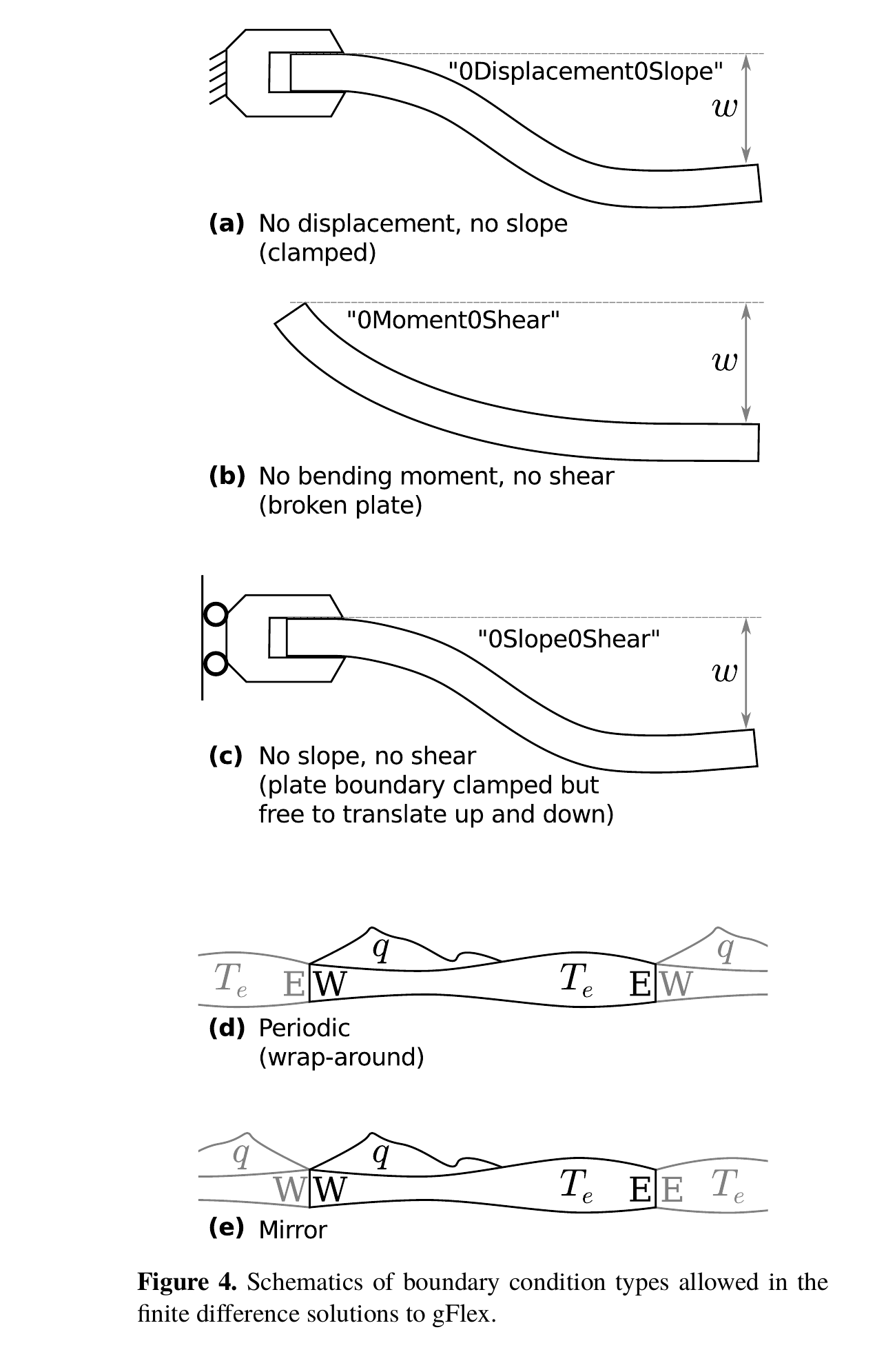
Schematics of five FD boundary condition types (a–e) from Wickert (2016), Fig. 4 (CC BY 3.0). zero_displacement_zero_moment (added post-publication) is not shown.

Tip

Flexural solutions can be sensitive to boundary conditions. When in doubt, use pad_domain() to push the boundaries far from the region of interest (works for both 1-D and 2-D), and choose zero_moment_zero_shear (free end) to minimise their influence.

---

Quantity names

The boundary condition names encode which plate mechanical quantities vanish at that edge. The table below maps each name component to its physical meaning and derivative order.

Quantity	Symbol	Definition (uniform \(D\), 1-D)	\(w\)-derivative order
Deflection	\(w\)	\(w\)	0th
Slope	\(S\)	\(\frac{\mathrm{d}w}{\mathrm{d}x}\)	1st
Bending moment	\(M\)	\(D\,\frac{\mathrm{d}^2 w}{\mathrm{d}x^2}\)	2nd
Shear force	\(V\)	\(D\,\frac{\mathrm{d}^3 w}{\mathrm{d}x^3}\)	3rd

---

Conditions

The table below summarises the five conditions. Detailed descriptions, geological context, and ball-and-stick diagrams appear in the sections below.

gFlex name	Zero at boundary	Structural mechanics	Geophysical	Description
zero_displacement_zero_slope (alias: clamped)	\(w\),\(S\)	clamped end	—	No deflection, no rotation
zero_displacement_zero_moment (alias: pinned)	\(w\),\(M\)	simply supported / pinned	—	No deflection, free to rotate
zero_moment_zero_shear (alias: free)	\(M\),\(V\)	free end	broken plate	Free, unsupported plate end
zero_slope_zero_shear (alias: mirror)	\(S\),\(V\)	—	mirror / symmetry	Even reflection; model half of a symmetric system
periodic	—	—	—	Domain wraps; opposite edges connected (per-axis pair for FFT)
no_outside_loads (alias: infinite)	—	—	semi-infinite plate	Auto-pad by ≥1 \(\alpha\); w trimmed to original domain

The “Geophysical” column reflects established usage in the lithospheric flexure literature. zero_moment_zero_shear is known as the “broken plate” condition; zero_slope_zero_shear (short alias mirror) is used under the symmetry-plane or mirror name in geophysical modeling. The remaining conditions are referred to by their structural-mechanics names, or have no name at all.

Deprecated since version 2.0: The v1.x PascalCase boundary-condition strings are no longer accepted. Rename them as follows:

Old name (v1.x)	New name (v2.0+)
0Displacement0Slope	zero_displacement_zero_slope
0Displacement0Moment	zero_displacement_zero_moment
0Moment0Shear	zero_moment_zero_shear
0Slope0Shear	zero_slope_zero_shear
Mirror	mirror
Periodic	periodic
NoOutsideLoads	no_outside_loads

---

zero_displacement_zero_slope

Zero displacement and zero slope: the plate is fully clamped at the boundary — no deflection and no rotation.

Standard names: clamped end (structural mechanics). No established geophysical name.

Geological context: No natural lithospheric analogue has been identified. The condition physically requires the plate to be rigidly anchored against both vertical movement and rotation at its edge, which has no clear counterpart in Earth’s lithosphere. In practice it serves as a conservative far-field constraint: when the domain boundary is placed far from any load and the plate is expected to be undisturbed there, clamping holds the plate at zero and zero slope — somewhat more conservative than the free-end condition at the same location. It is most appropriate as a boundary for a synthetic or test model, not as a representation of a physical plate edge.

Clamped end — zero deflection and zero slope at the boundary.

zero_displacement_zero_moment

Added in version 2.0.0.

Zero displacement and zero bending moment: the classical simply-supported (pinned) plate end. The plate is held at zero deflection but is free to rotate, so no moment is transmitted. Implemented as a Dirichlet condition (\(w = 0\)) at the boundary node and an odd-reflection ghost (\(w_\text{ghost} = -w_\text{interior}\)) at the first interior node to enforce zero curvature.

Standard names: simply supported or pinned end (structural mechanics). No established geophysical name.

Geological context: No natural lithospheric analogue has been identified. The condition is a mathematical convenience rather than a physical one: it is the natural condition for sine-series (Discrete Sine Transform) spectral solutions, where pinning both ends in deflection and freeing them in moment yields an odd-periodic extension that supports spectral computation without edge artefacts. Sine modes vanish at a simply-supported boundary; cosine modes vanish at a mirror boundary (see below).

Contrast with mirror

mirror and zero_displacement_zero_moment are both reflection boundary conditions but encode opposite parities. mirror uses an even reflection (\(w_\text{ghost} = +w_\text{interior}\)): the symmetry plane lies between the last real node and its ghost, the plate is horizontal at the boundary, and the deflection there is generally non-zero — making it the correct choice for modelling one half of a symmetric system. zero_displacement_zero_moment uses an odd reflection (\(w_\text{ghost} = -w_\text{interior}\)): the boundary node is the fixed point of the reflection, so \(w = 0\) there by definition, and the plate is free to rotate — the simply-supported end. Sine modes satisfy zero_displacement_zero_moment; cosine modes satisfy mirror.

Even reflection (mirror, left) vs. odd reflection (zero_displacement_zero_moment, right): the same four real nodes produce ghost values of opposite sign.

Simply supported — zero deflection, free to rotate; no bending moment transmitted.

zero_moment_zero_shear

The natural condition at a free edge: no bending moment and no shear force are transmitted across the boundary (Wickert, 2016, Table 1). Combined with an edge-applied load — a vertical point force supplies \(V_0\), a closely-spaced couple supplies \(M_0\) — it produces the classical broken-plate response of Turcotte and Schubert: the load carries the inhomogeneity through the loading vector while the BC matrix stays homogeneous.

Standard names: free end or free edge (structural mechanics); broken plate (geophysics). “Broken plate” is well established in the lithospheric flexure literature, referring to a plate whose edge is fractured and therefore transmits neither bending moment nor shear.

Geological context: zero_moment_zero_shear is the most physically motivated of the five conditions for Earth science applications:

• Passive or rifted continental margin, where the plate edge is effectively free

• Broken-plate flexure (Turcotte & Schubert) with an edge load applied at the boundary node

• Subduction trench and outer rise, where slab pull acts as an edge-applied vertical force

Free end — no bending moment and no shear force; the plate ends freely (“broken plate”).

zero_slope_zero_shear

Even reflection at the boundary: the system is identical on both sides, so only half the domain need be modelled. The deflection at the ghost node beyond the boundary equals the deflection at the corresponding interior node (\(w_\text{ghost} = +w_\text{interior}\)), the plate is horizontal at the boundary, and the deflection there is generally non-zero. Naturally compatible with cosine-series (Discrete Cosine Transform) solutions. For the distinction between even and odd reflections, see Contrast with mirror in the zero_displacement_zero_moment section above.

Short alias: mirror — accepted without any warning and normalised to zero_slope_zero_shear internally.

Standard names: No standard structural-mechanics or geophysical name. The condition is universally understood as a symmetry or mirror boundary.

Why the even-reflection ghost node enforces zero slope and zero shear: the rule \(w_\text{ghost} = +w_\text{interior}\) makes both the slope and the shear force vanish at the boundary automatically. In the central-difference stencil, the slope at the boundary node is

\[\frac{\mathrm{d}w}{\mathrm{d}x} \approx \frac{w_\text{interior} - w_\text{ghost}}{2\,\Delta x} = \frac{w_\text{interior} - w_\text{interior}}{2\,\Delta x} = 0,\]

and the third derivative (shear force) similarly cancels by the same even symmetry:

\[\frac{\mathrm{d}^3 w}{\mathrm{d}x^3} \approx \frac{w_{i+2} - 2w_{i+1} + 2w_{i-1} - w_{i-2}}{2\,\Delta x^3} \xrightarrow{w_{i-k}=w_{i+k}} 0.\]

The even-reflection ghost-node rule therefore simultaneously enforces \(\mathrm{d}w/\mathrm{d}x = 0\) and \(\mathrm{d}^3w/\mathrm{d}x^3 = 0\) — precisely the zero_slope_zero_shear prescription.

Geological context: zero_slope_zero_shear applies wherever the load and plate geometry are symmetric about the boundary plane:

• One flank of a mountain range, orogenic belt, or subduction trench

• One side of a continental ice sheet or ice cap

• Half of a foreland basin profile

• One quarter of a bilaterally symmetric ice dome or volcanic edifice (mirror on two perpendicular axes)

Symmetry plane — even reflection; use when the system is symmetric about the boundary.

periodic

Wrap-around: the domain tiles infinitely in the direction normal to that edge, and the solution wraps so that opposite edges are connected. Native to FFT-based spectral solutions, where periodicity is inherent to the transform.

For the FFT solver, periodic is applied per opposite-edge pair: setting both bc_west and bc_east to periodic makes the x-axis exactly periodic; setting both bc_north and bc_south to periodic makes the y-axis exactly periodic. Mixed axes are valid — for example, x-periodic and y-padded. A UserWarning is raised if only one side of a pair is periodic.

For the finite-difference solver a one-sided periodic is not well-posed and raises a ValueError; set allow_unpaired_periodic = True to override the guard and solve anyway (the deflection near that edge is not a valid solution).

Standard names: No standard structural-mechanics or geophysical name.

Geological context: periodic is appropriate when the load pattern genuinely repeats, or when the domain is large enough relative to the flexural wavelength that the periodic images of the load do not influence the region of interest:

• Seamount or volcanic chain

• Long linear load — mountain belt, fold-and-thrust belt, subduction trench, or rift system — where individual valley structure is below the flexural wavelength (though mirror at both flanks may be preferable for a bilaterally symmetric belt)

• Continental-scale glacial load

• Broad-scale FFT calculations

periodic — the domain wraps around; opposite edges are connected.

no_outside_loads

Added in version 2.0.0: Support for no_outside_loads in the finite-difference solver with automatic domain padding. For the FFT solver and the analytical (SAS / SAS_NG) methods, this is the native assumption and has always been available.

Short alias: infinite — accepted without any warning and normalised to no_outside_loads internally.

Emulates a plate that extends beyond the model domain with no loads applied outside. The finite-difference solver automatically pads the domain by at least one flexural wavelength (\(\lambda_\alpha = 2\pi\alpha\), where \(\alpha = (D / \Delta\rho\,g)^{1/4}\) is the flexural parameter) on each side where this condition is applied, solves on the extended domain with zero_displacement_zero_slope at the outer edge, then trims the result back to the original extent. The padding width and the solve are deterministic given the physical parameters, so the feature is safe to use in coupling loops.

no_outside_loads may be applied to any subset of edges — for example, west and east only while north and south use a different condition.

Geological context: no_outside_loads is the most physically appropriate FD condition when the load is entirely contained within the model domain and the surrounding lithosphere is unloaded. Natural choices include:

• Any self-contained load (seamount, ice cap, sedimentary basin)

• Coupling gFlex to a landscape evolution or ice-sheet model where the loaded region is surrounded by unloaded lithosphere

FFT and SAS: The FFT solver zero-pads non-periodic axes by default, which is equivalent to no_outside_loads for those axes. Explicitly setting FFT edges to no_outside_loads produces the same result and suppresses any partial-periodic warning. SAS / SAS_NG always assume no_outside_loads — it is the native assumption of the analytical superposition approach.

---

Prescribed (non-zero) boundary values

Added in version 2.0.0.

By default every boundary condition above enforces homogeneous constraints — the two named quantities are zero at the edge. The finite-difference solver also supports prescribed (non-zero) values by passing a dict in place of a BC string. This is the natural way to model a plate whose edge carries an applied load: for example, prescribing the shear force at a free end to represent slab pull at an ocean trench (the classical broken-plate scenario of Turcotte and Schubert, 2002), or setting a non-zero boundary displacement when coupling gFlex to another model.

This is available in F1D and F2D with method = 'fd'. Passing a dict BC to any other solver raises ValueError.

Relationship to string BCs

A dict BC uses the same finite-difference stencil as the equivalent string BC. The prescribed values enter as an additive correction to the right-hand side of the linear system — the coefficient matrix is unchanged. As a consequence, {"moment": 0.0, "shear": 0.0} produces exactly the same solution as the string "zero_moment_zero_shear": both constrain the same stencil structure and the RHS correction is zero. Only non-zero values change the solution.

Syntax

Set the BC attribute for a given edge to a dict with exactly two keys, where each key names a plate mechanical quantity and each value is either a scalar or a 1-D NumPy array:

flex.bc_west = {"moment": 0.0, "shear": V0}          # broken-plate edge load
flex.bc_west = {"displacement": 0.0, "slope": theta}  # prescribed rotation
flex.bc_east = {"displacement": w_array, "moment": 0.0}

The four valid keys are:

Key	Symbol	Prescribed quantity
"displacement"	\(w\)	Vertical deflection [m]
"slope"	\(dw/dx\)	Plate slope (dimensionless)
"moment"	\(M\)	Bending moment per unit edge length [N, i.e. N·m m⁻¹]
"shear"	\(V\)	Shear force per unit edge length [N m⁻¹]

Valid pairs

Each dict must contain exactly two keys whose combination corresponds to one of the four supported BC types:

Dict keys	Equivalent homogeneous BC
{"displacement", "slope"}	zero_displacement_zero_slope
{"displacement", "moment"}	zero_displacement_zero_moment
{"moment", "shear"}	zero_moment_zero_shear
{"slope", "shear"}	zero_slope_zero_shear

The two work-conjugate pairs — {"displacement", "shear"} and {"slope", "moment"} — are ill-posed and raise ValueError.

Array values (2-D only)

In 2-D, values may be 1-D arrays that vary along the edge. An array assigned to a north or south edge must have length equal to the number of columns; one assigned to a west or east edge must have length equal to the number of rows. Scalar values are broadcast to the full edge.

Example: broken-plate edge load (1-D)

The classical broken-plate scenario (Turcotte & Schubert, 2002) represents a semi-infinite oceanic plate carrying a vertical point force \(V_0\) at the trench end — the idealisation of slab pull at a subduction zone. The plate bends downward at the trench and a forebulge (outer rise) develops at approximately \(\pi\alpha/2\) from the loaded end.

The boundary condition is zero moment and prescribed (downward) shear at the west end, with a free zero_moment_zero_shear condition at the far east end:

import numpy as np
from gflex import F1D

# Physical parameters
E        = 65e9     # Pa — Young's modulus
nu       = 0.25
rho_m    = 3300.0   # kg m⁻³ — mantle density
rho_fill = 0.0      # kg m⁻³ — air infill
g        = 9.8      # m s⁻²
Te       = 30e3     # m  — elastic thickness

# Derived quantities
D     = E * Te**3 / (12.0 * (1.0 - nu**2))          # flexural rigidity
lam   = ((rho_m - rho_fill) * g / (4.0 * D)) ** 0.25
alpha = 1.0 / lam                                    # flexural parameter ≈ 66 km

# Domain: 10 α long, 401 nodes
nx = 401
dx = 10.0 * alpha / (nx - 1)

# Slab-pull shear force at the trench (negative = downward), N/m
V0 = -1e12

flex = F1D()
flex.quiet    = True
flex.method   = 'fd'
flex.g = g;  flex.E = E;  flex.nu = nu
flex.rho_m = rho_m;  flex.rho_fill = rho_fill
flex.T_e      = Te
flex.qs       = np.zeros(nx)   # no distributed load — forcing is at the boundary
flex.dx       = dx
flex.bc_west  = {"moment": 0.0, "shear": V0}   # trench: zero moment, prescribed shear
flex.bc_east  = "zero_moment_zero_shear"         # free far end

flex.initialize()
flex.run()
w = flex.w   # deflection [m]; w[0] ≈ −933 m (trench), forebulge ≈ +63 m at x ≈ 156 km
flex.finalize()

The result matches the analytical solution \(w(x) = \frac{V_0}{2D\lambda^3}\,e^{-\lambda x}\cos(\lambda x)\) to within 0.02 % (L-∞ relative error).

A standalone version of this script with plotting is provided in input/run_in_script_prescribed_bc_1D.py.