Numerical Accuracy

Each solution method in gFlex has a distinct accuracy profile.

Analytical solutions (sas and sas_ng)

The superposition-of-analytical-solutions methods are exact for a plate of constant elastic thickness under the no_outside_loads boundary condition (zero deflection at infinity). In one dimension the Green’s function is the exponential sinusoid of Eq. (3) in Wickert (2016); in two dimensions it is the zeroth-order Kelvin function \(\mathrm{kei}\), evaluated via scipy.special.kei(). Floating-point errors in these special-function evaluations are at machine precision and negligible in practice.

The only meaningful source of error is a domain that is too small: if the load produces non-trivial deflection at the domain boundary, the no_outside_loads assumption is violated and the solution is physically wrong — not because of numerics, but because the boundary condition does not match the situation. Use gflex.flexural_wavelengths() to estimate the flexural parameter \(\alpha\) and ensure the domain extends several \(\alpha\) beyond the loaded region. Unlike the finite difference solver, there is no grid-spacing error; output sampling density affects only the display, not the solution.

FFT spectral solver

The FFT solver is spectrally accurate for uniform elastic thickness: for a smooth load field the solution error decays faster than any finite power of the grid spacing, limited in practice only by floating-point arithmetic. For periodic boundary conditions (periodic on all sides) the solution is exact to machine precision. For all other boundary conditions the load is zero-padded by \(4\alpha\) on each side before the transform, which approximates the no_outside_loads condition; the padding introduces a small error near the domain edges that decreases as the pad width increases relative to the load’s flexural footprint. For typical geoscience applications the \(4\alpha\) default padding is more than sufficient.

Because the FFT assumes a single, spatially uniform flexural rigidity \(D\), it cannot represent variable-\(T_e\) problems; those require the finite difference solver.

Finite difference solver (fd)

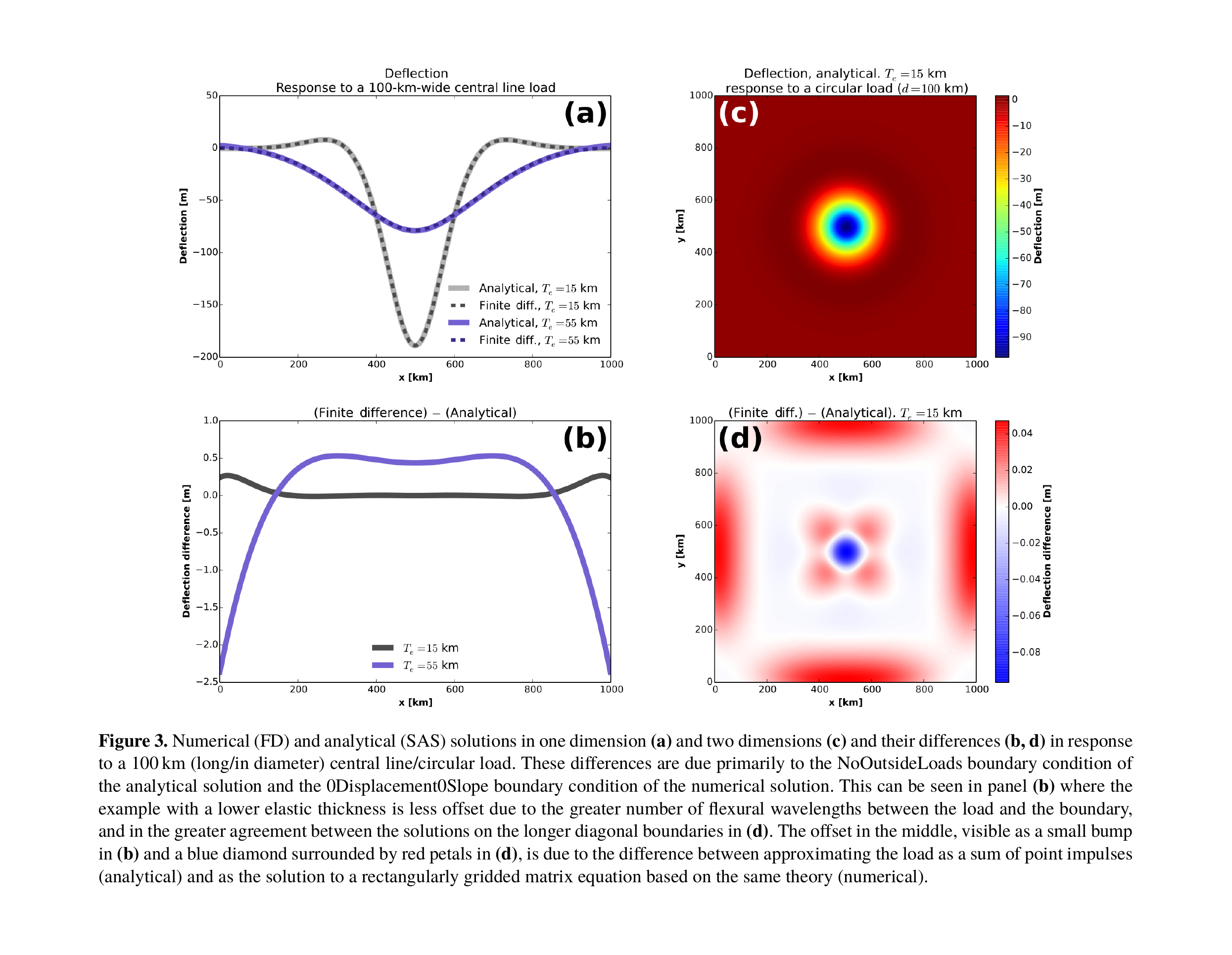
Comparison of numerical (FD) and analytical (SAS) solutions in one dimension (a) and two dimensions (c), and their differences (b, d), for a 100 km central line load / circular load. The 1–2 m offset in (b) is due primarily to the no_outside_loads BC of the analytical solution versus the zero_displacement_zero_slope BC of the FD solution; the cross-shaped residual in (d) reflects boundary effects along the longer diagonal boundaries. Reproduced from Wickert (2016), Fig. 3; CC BY 3.0.

---

2-D finite-difference solver: second-order convergence

The 2-D finite-difference solver (method = 'fd') is second-order accurate in space: halving the grid spacing \(\Delta x\) reduces the numerical error by a factor of approximately four (\(\mathcal{O}(\Delta x^2)\)).

This is verified two ways in gFlex:

1. Method of Manufactured Solutions (MMS) — a formal unit test (tests.test_2D_FD.test_2d_fd_convergence_order()) that runs with every CI build. A cosine deflection field is chosen as the exact solution; the corresponding load is derived analytically and fed to the solver. Three grid refinements (N = 30, 60, 120 cells per side) on a periodic domain confirm a convergence rate > 1.8 at all refinement levels.

2. Kelvin-function benchmark — a grid-convergence study comparing the FD solver to the analytical Kelvin-function solution for an infinite plate under a point load. Results are summarised in the table below.

Kelvin-function benchmark setup

Young’s modulus \(E\)	65 GPa
Elastic thickness \(T_e\)	10 km
Poisson’s ratio \(\nu\)	0.25
Mantle density \(\rho_m\)	3300 kg m⁻³
Infill density \(\rho_\text{fill}\)	0 kg m⁻³ (air)
\(g\)	9.81 m s⁻²
Flexural parameter \(\alpha\)	≈ 21 km
Domain	600 km × 600 km, point load at centre
Boundary conditions	zero_moment_zero_shear on all four sides
Grid spacings tested	\(\Delta x\) = 10 000, 5 000, 2 500, 1 250 m

Convergence orders (coarse → fine)

The table gives the local convergence order between successive grid refinements at several distances from the load, expressed as multiples of the flexural parameter α.

\(r/\alpha\)	\(\Delta x\) 10→5 km	\(\Delta x\) 5→2.5 km	\(\Delta x\) 2.5→1.25 km
0.97	2.20	2.07	2.01
1.46	2.68	2.18	2.04
1.95	1.07	1.88	1.97
2.92	−0.07	1.77	1.95

At the finest spacing (\(\Delta x = 1250\) m, \(\Delta x/\alpha \approx 0.06\)) relative errors are 0.02–0.1 % everywhere except very close to the singularity of the point load.

The sub-second-order rates at \(r/\alpha\) = 1.95 and 2.92 on the coarsest grids reflect pre-asymptotic effects near the forebulge zero-crossing, where the solution changes sign and the absolute error temporarily dominates the relative error. All rates converge to ≈ 2 at finer resolution, confirming asymptotic second-order behaviour.

Practical guidance

For most geoscience applications, \(\Delta x / \alpha \leq 0.1\) (ten cells per flexural parameter) is sufficient to keep errors below 1 %. At \(\Delta x / \alpha \approx 0.5\) (two cells per flexural parameter) errors can be several percent, particularly near the load centre and the forebulge. Use gflex.flexural_wavelengths() to estimate \(\alpha\) before choosing a grid spacing.

---

1-D zero_displacement_zero_slope boundary condition: ghost-node correction (2026)

Left: Deflection profiles at \(\Delta x = 3\) km; exact (MMS), corrected, and original implementations are indistinguishable at this scale. Centre: Residuals (numerical − exact). The original implementation has a systematic error that grows toward the boundaries; the corrected implementation is everywhere within floating-point noise. Right: Convergence with grid refinement. The original implementation converges at \(\mathcal{O}(\Delta x^{0.97})\) — first order — while the corrected implementation achieves \(\mathcal{O}(\Delta x^{2.0})\), consistent with the interior stencil.

Background

The zero_displacement_zero_slope (clamped) finite-difference boundary condition requires the elimination of two ghost nodes outside the domain at each end of the plate. In a clamped (zero-slope) condition, the ghost node immediately outside the boundary satisfies an even reflection:

\[w_{-1} = w_{+1} \quad\text{(west end)}\]

rather than the odd reflection used by the zero-moment (zero-curvature) condition. Additionally, the boundary row itself must be decoupled from interior nodes so that the linear system directly enforces \(w_0 = 0\) as a Dirichlet constraint.

The original implementation (present since gFlex 1.0, 2016) dropped ghost nodes by setting them to NaN rather than eliminating them via even reflection, and did not decouple the boundary row. As a result:

• \(w_0\) was not strictly zero — the linear system retained off-diagonal coupling that allowed the boundary value to drift.

• The zero-slope condition was not enforced at the discrete level.

• The convergence rate was \(\mathcal{O}(\Delta x)\) rather than \(\mathcal{O}(\Delta x^2)\).

MMS verification

The error is quantified with a Method of Manufactured Solutions (MMS) test. The exact solution

\[w_\mathrm{exact}(\xi) = -W_0\,\xi^2\,(1-\xi)^2, \quad \xi = x/L,\]

satisfies both boundary conditions at \(\xi = 0\) and \(\xi = 1\) exactly (\(w = 0\), \(dw/d\xi = 0\)). Its fourth derivative is constant, so the manufactured load

\[q_s(\xi) = \frac{24\,D\,W_0}{L^4} + \Delta\rho\,g\,W_0\,\xi^2(1-\xi)^2\]

includes a spatially varying elastic-foundation term — making this a nontrivial test of the full governing equation, not just the biharmonic operator alone.

The error metric is the \(L^\infty\) relative error:

\[e = \frac{\max|w_\mathrm{num} - w_\mathrm{exact}|} {\max|w_\mathrm{exact}|}\]

Physical parameters used: \(T_e = 30\) km, \(E = 65\) GPa, \(\nu = 0.25\), \(\rho_m = 3300\) kg m⁻³, \(\rho_\mathrm{fill} = 0\), \(g = 9.81\) m s⁻², \(L = 600\) km.

Results

\(n_x\)	\(\Delta x\) [km]	original error	corrected error	factor
26	24.0	4.34 × 10⁻²	1.84 × 10⁻³	24×
51	12.0	2.75 × 10⁻²	4.55 × 10⁻⁴	60×
101	6.0	1.54 × 10⁻²	1.14 × 10⁻⁴	135×
201	3.0	8.11 × 10⁻³	2.85 × 10⁻⁵	285×
401	1.5	4.16 × 10⁻³	7.12 × 10⁻⁶	584×
801	0.75	2.11 × 10⁻³	1.78 × 10⁻⁶	1184×

Convergence slopes (finest three points): original \(\mathcal{O}(\Delta x^{0.97})\); corrected \(\mathcal{O}(\Delta x^{2.00})\). The boundary value \(w[0]\) (exactly zero in the MMS solution) was \(-4.9 \times 10^{-3}\) m in the original and \(-1.6 \times 10^{-8}\) m in the corrected implementation at \(\Delta x = 0.75\) km.

Under an interior-only point load (\(q_s[0] = q_s[N-1] = 0\)), the corrected Dirichlet decoupling enforces \(w[0] = 0\) exactly: with all off-diagonal stencil entries at the boundary node removed and zero load on the boundary, the boundary equation reduces to \(c_0 w[0] = 0\). The original implementation gives \(w[0] \approx +1.1 \times 10^{-4}\) m at \(\Delta x = 3\) km.

Practical impact

The original implementation gave acceptably small errors when the boundary was far from any load — the intended use case, reinforced by the zero_displacement_zero_slope proximity warning added in gFlex 1.4. When a load was placed close to a clamped boundary, the first-order error could produce boundary deflections of order \(10^{-3}\) relative to the maximum deflection. For a 1 km deflection this corresponds to roughly 1 mm of spurious boundary motion — negligible in most geoscience applications, but detectable in high-resolution model comparisons.

The correction is in commit 6f68270 (not present in gFlex 1.4.0). See the Release Notes for the full bug-fix note.

The standalone error-analysis script is at analysis/analyze_clamped_bc_error.py, and a git-worktree–based cross-version comparator is at analysis/compare_bc_versions.py.

---

1-D and 2-D zero_moment_zero_shear boundary condition: ghost-node correction (2026)

Left: Deflection profiles at \(\Delta x = 3\) km; exact (MMS), corrected, and original implementations are nearly indistinguishable at this scale. Centre: Residuals (numerical − exact). The original implementation has a systematic error that decays slowly toward the boundaries; the corrected implementation is well within the second-order truncation error envelope. Right: Convergence with grid refinement. The original implementation converges at \(\mathcal{O}(\Delta x^{0.99})\) — first order — while the corrected implementation achieves \(\mathcal{O}(\Delta x^{2.00})\), consistent with the interior stencil.

2-D analogue of the 1-D figure above (centre row shown). The convergence rates are the same: \(\mathcal{O}(\Delta x^{0.94})\) for the original and \(\mathcal{O}(\Delta x^{2.01})\) for the corrected implementation over the tested resolution range.

Background

The zero_moment_zero_shear (free broken-end) boundary condition requires eliminating one ghost node at each end of the plate. The boundary node (i=0) uses both the moment condition (\(d^2w/dx^2 = 0 \Rightarrow w_{-1} = 2w_0 - w_1\)) and the shear condition (\(d^3w/dx^3 = 0 \Rightarrow w_{-2} = 4w_0 - 4w_1 + w_2\)). The first interior node (i=1) also has a ghost \(w_{-1}\) in its five-point stencil that must be eliminated.

The original implementation eliminated this ghost using the shear condition evaluated at the staggered location \(x = \Delta x\) (one cell inward from the boundary):

\[\frac{d^3w}{dx^3}\bigg|_{x=\Delta x} = 0 \quad\Longrightarrow\quad w_{-1} = 2w_0 - 2w_2 + w_3\]

This is internally inconsistent: both the boundary row and the first interior row eliminate the same ghost \(w_{-1}\), but using different physical conditions evaluated at different points. For homogeneous BCs (M = V = 0) the inconsistency is invisible, but it introduces a non-standard truncation error at i=1.

The corrected implementation uses the same moment condition at both rows:

\[\frac{d^2w}{dx^2}\bigg|_{x=0} = 0 \quad\Longrightarrow\quad w_{-1} = 2w_0 - w_1\]

which is the physically correct constraint for the node immediately inside the boundary. All four edges (west j=1, east j=N-2, north i=1, south i=N-2) required the same three-line correction in the 2-D solver.

MMS verification

The manufactured solution

\[w_\mathrm{exact}(\xi) = -W_0\,\xi^4\,(1-\xi)^4, \quad \xi = x/L,\]

satisfies all four free-end boundary conditions (\(w''=w'''=0\)) at both ends exactly. Its fourth derivative is

\[\frac{d^4 w}{dx^4} = -\frac{W_0}{L^4} \bigl(24 - 480\xi + 2160\xi^2 - 3360\xi^3 + 1680\xi^4\bigr),\]

giving the manufactured load

\[q_s(\xi) = \frac{D\,W_0}{L^4} \bigl(24 - 480\xi + 2160\xi^2 - 3360\xi^3 + 1680\xi^4\bigr) + \Delta\rho\,g\,W_0\,\xi^4(1-\xi)^4.\]

The 2-D extension uses the separable solution \(w = -W_0\,f(\xi)\,f(\eta)\) with \(f(t) = t^4(1-t)^4\), which satisfies the free-end condition on all four sides.

Physical parameters used: \(T_e = 30\) km, \(E = 65\) GPa, \(\nu = 0.25\), \(\rho_m = 3300\) kg m⁻³, \(\rho_\mathrm{fill} = 0\), \(g = 9.81\) m s⁻², \(L = 600\) km, \(W_0 = 25600\) m (giving \(|w_\mathrm{exact}|_\mathrm{max} = 100\) m).

Results (1-D)

\(n_x\)	\(\Delta x\) [km]	original error	corrected error	factor
26	24.0	9.00 × 10⁻²	1.72 × 10⁻²	5×
51	12.0	6.97 × 10⁻²	4.40 × 10⁻³	16×
101	6.0	3.90 × 10⁻²	1.11 × 10⁻³	35×
201	3.0	2.02 × 10⁻²	2.77 × 10⁻⁴	73×
401	1.5	1.02 × 10⁻²	6.93 × 10⁻⁵	148×
801	0.75	5.14 × 10⁻³	1.73 × 10⁻⁵	297×

Convergence slopes (finest three points): original \(\mathcal{O}(\Delta x^{0.99})\); corrected \(\mathcal{O}(\Delta x^{2.00})\).

Results (2-D)

\(n_x = n_y\)	\(\Delta x\) [km]	original error	corrected error	factor
26	24.0	8.73 × 10⁻²	1.76 × 10⁻²	5×
51	12.0	6.88 × 10⁻²	4.53 × 10⁻³	15×
101	6.0	3.95 × 10⁻²	1.15 × 10⁻³	34×
201	3.0	2.06 × 10⁻²	2.85 × 10⁻⁴	72×

Convergence slopes (finest two points): original \(\mathcal{O}(\Delta x^{0.94})\); corrected \(\mathcal{O}(\Delta x^{2.01})\).

Boundary exactness

Because the boundary-node equation (i=0) is identical in the original and corrected implementations — both apply the moment and shear ghost conditions the same way at the plate edge — both satisfy \(d^2w/dx^2 = 0\) and \(d^3w/dx^3 = 0\) to machine precision at the boundary node. The finite- difference estimates of moment and shear at the edge are \(\lesssim 10^{-12}\) m m⁻² and \(\lesssim 10^{-17}\) m m⁻³ for both implementations under an interior-only point load.

The original code’s error is at i=1, where the staggered shear ghost introduces a non-standard truncation error. Under an interior point load at \(\Delta x = 3\) km, the first-interior-node displacement differs by \(|w_\mathrm{old}[1] - w_\mathrm{new}[1]| \approx 5.5 \times 10^{-4}\) m between old and new — it is this node-level discrepancy that accumulates to produce the \(\mathcal{O}(\Delta x)\) convergence shown above.

Practical impact

The original implementation degraded the convergence rate of the zero_moment_zero_shear boundary from second order to first order. In practice, the error is largest when the domain is short relative to the flexural parameter \(\alpha\) — which is unlikely in typical geoscience use, where free-end BCs are most appropriate for long rifted margins or spreading ridges that extend well beyond the loaded region. The degradation is also self-consistent for homogeneous BCs (M = V = 0), so the absolute error is often acceptable. However, the first-order convergence meant that refining the grid to improve accuracy was less efficient than expected.

The correction (issues #62 and #63) is in commits b7eecc8 (1-D) and c117ccd (2-D).

The standalone error-analysis script is at analysis/analyze_free_end_bc_error.py.

---

2-D zero_displacement_zero_slope boundary condition: ghost-node correction (2026)

Left: Deflection profiles along the centre row at \(\Delta x = 6\) km; exact (MMS), corrected, and original implementations are nearly indistinguishable at this scale. Centre: Residuals (numerical − exact) along the centre row. The original implementation has a systematic error that grows toward the boundaries; the corrected implementation is well within the second-order truncation error envelope. Right: Convergence with grid refinement. The original implementation converges at \(\mathcal{O}(\Delta x^{0.92})\); the corrected implementation achieves \(\mathcal{O}(\Delta x^{1.99})\), consistent with the interior stencil.

Background

The 2-D zero_displacement_zero_slope (clamped) boundary condition carries the same two ghost-node bugs that were present in the 1-D code:

1. Boundary column/row not decoupled. Off-diagonal stencil entries at the boundary column (or row) were left at their interior stencil values — that is, the boundary nodes retained coupling to interior nodes rather than being set as strict Dirichlet constraints with \(w = 0\).

2. Even-reflection ghost missing. The first interior column (or row) requires the even-reflection ghost \(w[-1, i] = w[1, i]\) (for a west boundary) to enforce zero slope at the grid level. The original code left this ghost out, so the zero-slope condition was only approached asymptotically rather than being imposed algebraically.

These are the 2-D counterparts of the 1-D issues described in the preceding section. The north and south blocks additionally contained [!= inf] = nan patterns that, while harmless in practice (those entries land outside the assembled matrix range), obscured the logic and have been replaced with consistent += np.inf assignments.

MMS verification

The error is quantified with a Method of Manufactured Solutions (MMS) test. The exact solution

\[w_\mathrm{exact}(\xi, \eta) = -W_0\, g(\xi)\, g(\eta), \quad g(t) = t^2(1-t)^2, \quad \xi = x/L,\ \eta = y/L,\]

satisfies all four clamped boundary conditions (\(w = 0\), \(\partial w/\partial n = 0\)) exactly. Because \(g''''(t) = 24\) (constant), the manufactured load

\[q_s(\xi,\eta) = \frac{D\,W_0}{L^4} \bigl[24\,g(\eta) + 2\,g''(\xi)\,g''(\eta) + 24\,g(\xi)\bigr] + \Delta\rho\,g\,W_0\,g(\xi)\,g(\eta)\]

includes a spatially varying elastic-foundation term, making this a nontrivial test of the full governing equation.

The error metric is the \(L^\infty\) relative error:

\[e = \frac{\max|w_\mathrm{num} - w_\mathrm{exact}|} {\max|w_\mathrm{exact}|}\]

Physical parameters: \(T_e = 30\) km, \(E = 65\) GPa, \(\nu = 0.25\), \(\rho_m = 3300\) kg m⁻³, \(\rho_\mathrm{fill} = 0\), \(g = 9.81\) m s⁻², \(L = 600\) km, \(W_0 = 1600\) m (max \(|w_\mathrm{exact}| = 6.25\) m).

Results

\(n_x = n_y\)	\(\Delta x\) [km]	original error	corrected error	factor
26	24.0	3.98 × 10⁻²	1.61 × 10⁻³	25×
51	12.0	2.60 × 10⁻²	4.31 × 10⁻⁴	60×
101	6.0	1.47 × 10⁻²	1.10 × 10⁻⁴	134×
201	3.0	7.78 × 10⁻³	2.75 × 10⁻⁵	283×

Convergence slopes (finest two points): original \(\mathcal{O}(\Delta x^{0.92})\); corrected \(\mathcal{O}(\Delta x^{1.99})\).

Under an interior-only point load (zero load on all boundary rows and columns), the corrected implementation gives \(\max|w| = 0\) exactly on all four boundary edges; the original gives \(\max|w| \approx 2.2 \times 10^{-4}\) m at \(n = 51\) (\(\Delta x = 12\) km).

Practical impact

As with the 1-D case, the original 2-D zero_displacement_zero_slope implementation gave acceptably small errors when the clamped boundary was far from any load — the intended use case. The error grew near the boundary and converged at only first order, meaning grid refinement was less efficient than expected. The correction enforces the Dirichlet constraint algebraically and recovers full second-order convergence on all four sides.

The correction is in commit 984f7a4.

The standalone error-analysis script (covering both 1-D and 2-D) is at analysis/analyze_clamped_bc_error.py.