Example: Greenland

This page works through two related problems using Greenland as the study area. The first is a realistic model of present-day lithospheric deflection under the Greenland ice sheet, using publicly available ice-thickness and elastic-thickness datasets. The second is a hypothetical extension that uses the regional model as the starting point for a finer-scale nested solve, specifically to illustrate how inhomogeneous (prescribed-value) boundary conditions let a local model inherit its boundary state from a coarser regional solve. A Gaussian seamount — purely hypothetical — is then added to the local model to show how a new coastal load perturbs the plate on top of the existing ice-sheet deformation field.

Scripts: examples/greenland_flexure.py (regional model) and examples/greenland_volcano_nested.py (nested model).

Datasets

Both scripts draw on the same two datasets.

Ice thickness — BedMachine Greenland v6 (Morlighem et al. 2017, 2025), available from NSIDC (Earthdata login required). The native 150 m grid is subsampled to ~10 km before passing to gFlex; at that resolution each FD solve takes a few seconds.

Elastic thickness — Steffen et al. (2018, 2026), freely available under CC-BY-4.0 from Zenodo (doi:10.5281/zenodo.18403685). The script downloads this file automatically on first run. The dataset provides \(T_e\) in km at 0.2° geographic spacing over the greater Greenland region; values range from 5 to 87 km, reflecting the contrast between the weak western margin and the cratonic interior.

Regional ice-sheet model

Setup

The BedMachine grid is already in EPSG:3413 (NSIDC Sea Ice Polar Stereographic North). The Steffen et al. data is in geographic lon/lat and must be reprojected onto the same EPSG:3413 grid using pyproj and scipy.interpolate.RegularGridInterpolator. Cells outside the Te dataset coverage are assigned the domain median.

Only grounded ice (BedMachine mask == 2) contributes to the surface load; floating ice is hydrostatically supported by the ocean and is excluded. The load is \(q_s = \rho_\text{ice}\,g\,H_\text{ice}\) with \(\rho_\text{ice} = 917\) kg m⁻³.

Boundary conditions and domain padding

A clamped boundary condition (zero_displacement_zero_slope) is applied on all four sides. This requires that deflections approach zero before the domain edge — enforced here by calling pad_domain() with one flexural wavelength of padding (~650 km for the mean \(T_e\) of 46 km). The padding ring tapers \(T_e\) smoothly to the domain mean and carries zero load; after the solve the padding is trimmed from w with w = flex.w[p:-p, p:-p].

Without padding the forebulge reached 61 m; with padding it is 36 m, confirming that free-end boundary artefacts were inflating the unpadded result.

from gflex import F2D, pad_domain

te_pad, qs_pad, p = pad_domain(te_proj, qs, dx=dx, dy=dy,
                                E=65e9, nu=0.25, rho_m=3300., g=9.81)
flex = F2D()
flex.T_e, flex.qs = te_pad, qs_pad
flex.dx, flex.dy = dx, dy
flex.bc_west = flex.bc_east = flex.bc_north = flex.bc_south = \
    'zero_displacement_zero_slope'
flex.initialize()
flex.run()
w = flex.w[p:-p, p:-p]   # trim padding

Results

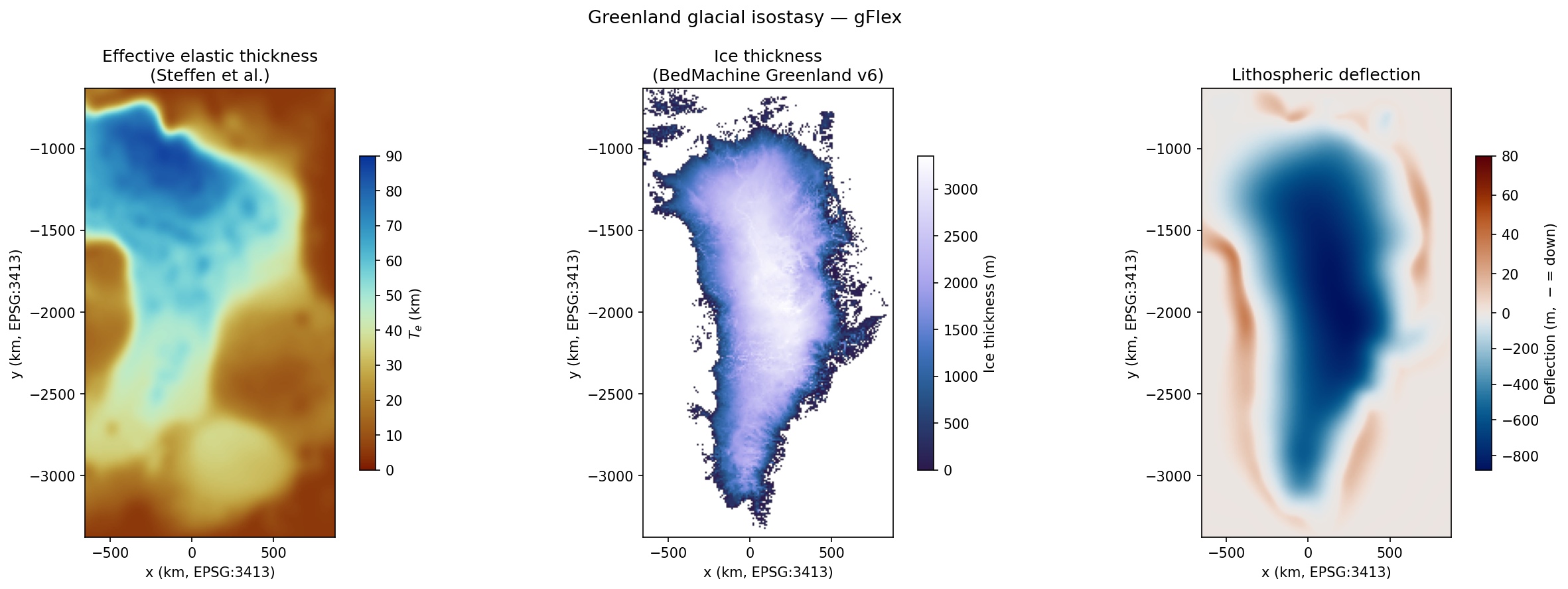
Left: effective elastic thickness \(T_e\) (Steffen et al.; roma colormap). Centre: ice thickness from BedMachine v6 (grounded ice only; devon colormap). Right: computed lithospheric deflection (vik colormap, asymmetric scale: blue = subsidence, red = uplift).

The maximum depression is 880 m beneath the central ice dome. The forebulge reaches 36 m and is notably sharp along the east coast, where \(T_e\) drops steeply from the cratonic interior toward the passive margin. That abrupt change in plate stiffness concentrates the bending and narrows the forebulge wavelength.

Effect of spatially variable \(T_e\)

Running a second solve with \(T_e\) fixed at the ice-sheet mean (46 km everywhere) isolates the contribution of lateral heterogeneity.

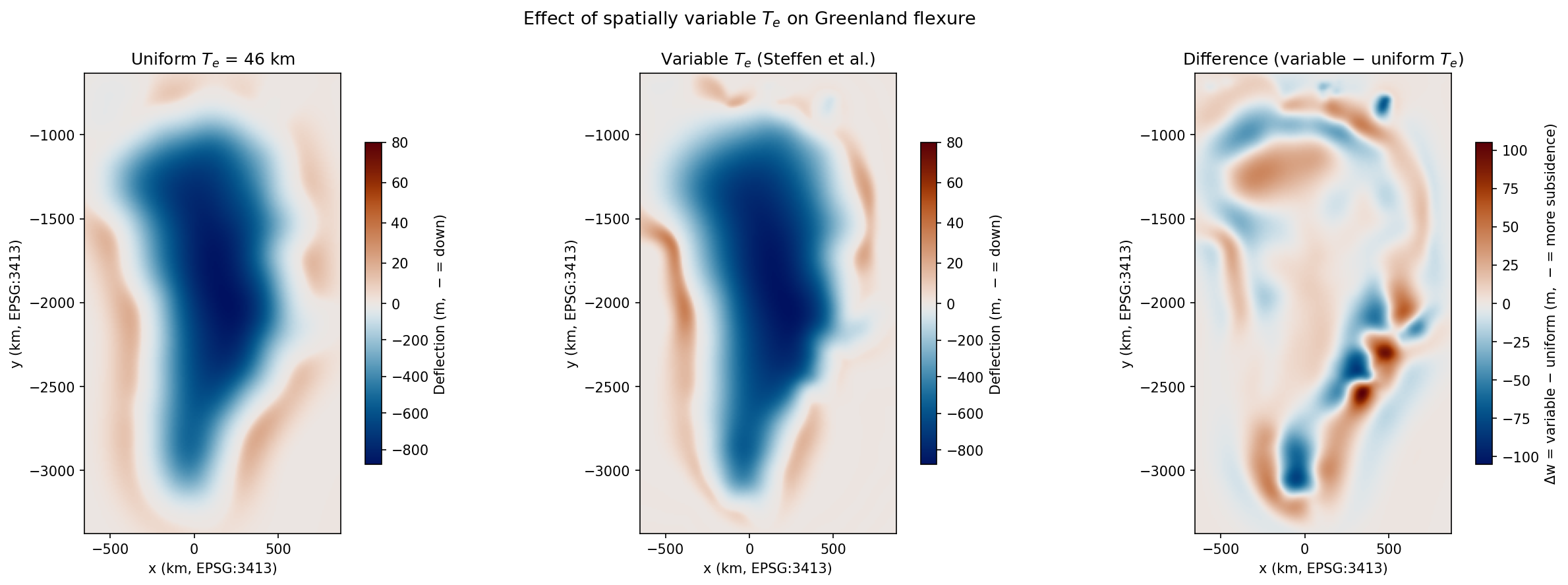
Left: deflection under uniform \(T_e\) = 46 km. Centre: deflection under the spatially variable Steffen et al. \(T_e\). Right: difference (variable − uniform); red = variable \(T_e\) produces more subsidence (locally weak lithosphere), blue = less subsidence (locally strong lithosphere).

The two total depressions agree within 1 m (both ~880 m), because the load magnitude is dominated by the thick central ice, which sits on near-average \(T_e\). The differences are largest at the margins: up to +105 m (more subsidence) where \(T_e\) dips well below the mean along the western coast, and up to −85 m (less subsidence) over the strong cratonic keel in the southeast. For a regional model used to infer ice-loading history or present-day rebound rates, assuming a uniform \(T_e\) would introduce errors of this magnitude at the margins.

Nested-domain model: a hypothetical coastal seamount

The regional model sets up a physically meaningful background state — a plate already stressed by several hundred metres of ice-sheet deflection — against which the effect of a new local load can be evaluated. This second example uses that background to illustrate how inhomogeneous boundary conditions couple a coarse regional model to a fine local one.

The scenario is hypothetical: a Gaussian seamount (\(h_\text{peak} = 2\) km, \(\sigma = 20\) km) appears on the SE Greenland coast near ~64°N 40°W. The fine sub-domain is 300 × 300 km at 2 km resolution, centred where the ice margin, the forebulge, and the open ocean all fall within a single window.

Extracting boundary conditions from the regional model

The fine model’s boundary state comes entirely from the coarse solution. At each of the four edges, displacement and slope are sampled with scipy.interpolate.RegularGridInterpolator and passed directly to F2D:

import numpy as np
from scipy.interpolate import RegularGridInterpolator

dw_dx = np.gradient(w_coarse, dx, axis=1)   # dw/dx, positive = eastward
dw_dy = np.gradient(w_coarse, dy, axis=0)   # dw/dy, positive = southward

# sample at fine-domain edge coordinates via RegularGridInterpolator ...

flex_fine.bc_west  = {"displacement": w_west,  "slope": dw_dx_west}
flex_fine.bc_east  = {"displacement": w_east,  "slope": dw_dx_east}
flex_fine.bc_north = {"displacement": w_north, "slope": dw_dy_north}
flex_fine.bc_south = {"displacement": w_south, "slope": dw_dy_south}

The slope convention is the same on all four edges: the value passed as "slope" is \(\mathrm{d}w/\mathrm{d}x\) (for west and east) or \(\mathrm{d}w/\mathrm{d}y\) in the row-index direction, positive southward (for north and south). Both are obtained from numpy.gradient() with positive grid spacings. This convention is verified by the round-trip unit test TestNestedModelGradientRoundTrip in tests/test_2D_inhomogeneous_BC.py, which confirms that a sub-domain re-solve with gradients extracted from a full solve reproduces the full-domain interior to within the accuracy of the finite difference gradient estimate.

The ice load within the fine domain is resampled from the coarse grid to 2 km and included explicitly in the fine solve, so the boundary conditions supply the far-field constraint while the local ice drives the near-field plate response.

Results

Both fine-domain results are new, independent finite-difference solutions on the 2 km grid — not subsamplings or interpolations of the coarse result. The prescribed displacement and slope at each boundary encode the cumulative plate response to the entire ice sheet, including the bulk of the Greenland load that lies well outside the fine window. A homogeneous boundary condition (e.g., clamped or free edges) would ignore that far-field loading and give a physically wrong answer even in the domain interior. Two solves are run with identical boundary conditions: one with ice load only (background) and one with ice plus the seamount load (total). Their difference isolates the volcanic signal.

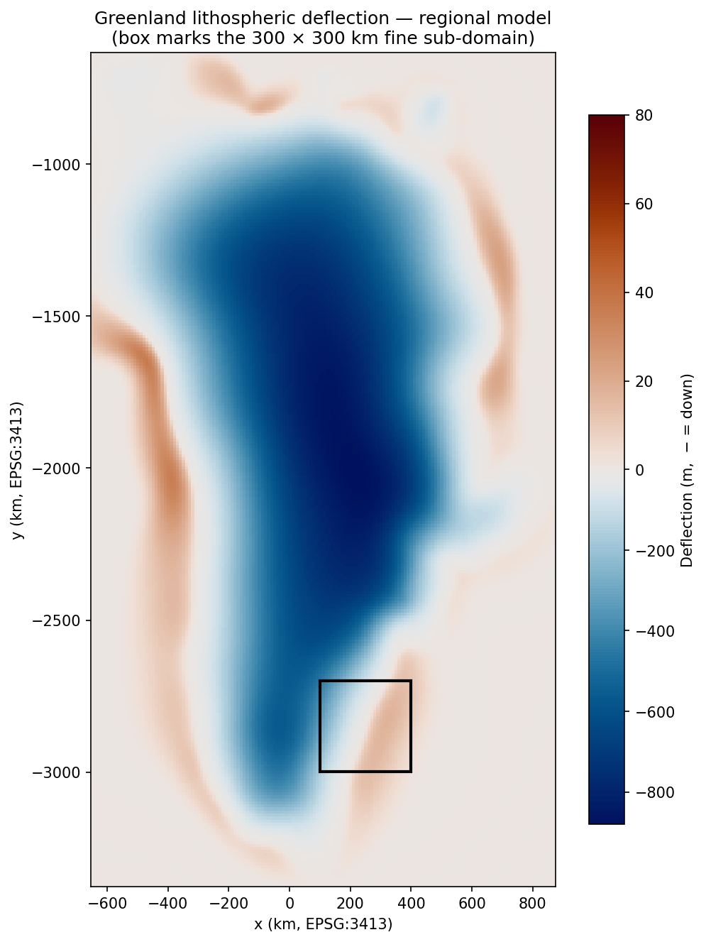
Regional Greenland lithospheric deflection (vik colormap, same scale as the regional model above). The black box marks the 300 × 300 km fine sub-domain centred on the SE Greenland coast (~64°N 40°W), straddling the ice-sheet margin and the forebulge.

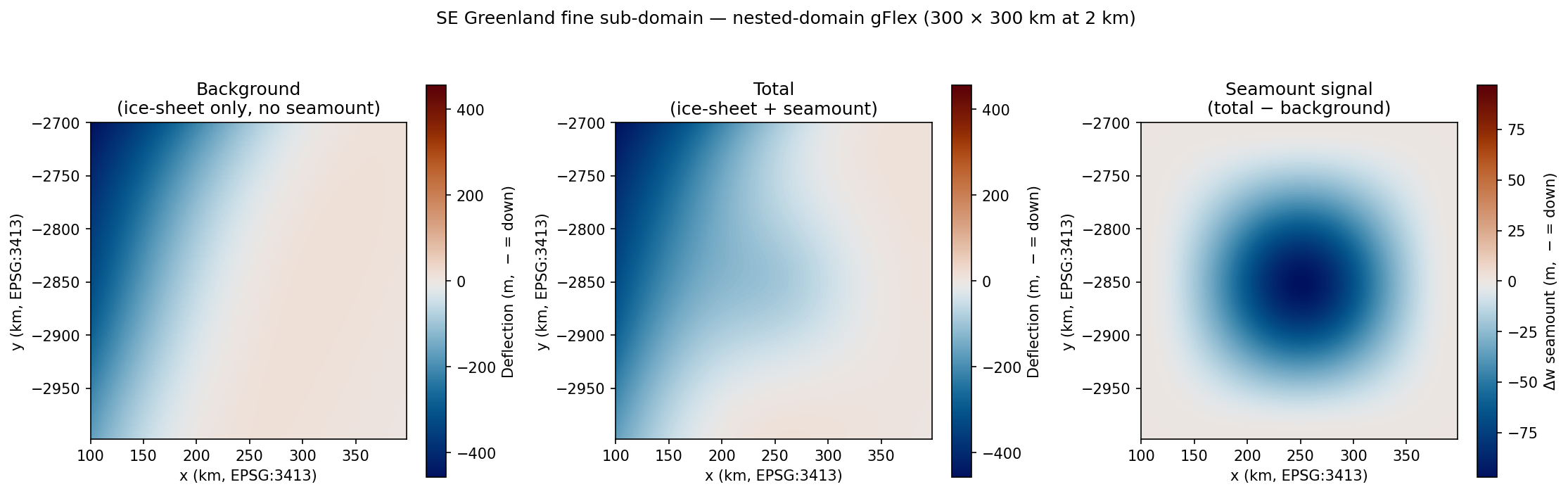
Left: fine-model background — the transition from ice-sheet depression (west, over grounded ice) to forebulge (east, open ocean) is clearly visible within the single 300 km window. Centre: total fine deflection (ice-sheet + seamount); the circular volcanic depression is superimposed on the ice-sheet pattern. Right: isolated seamount signal (total − background); 97 m central depression with no measurable forebulge, consistent with the sub-flexural load width (\(\sigma = 20\) km \(\ll \alpha \approx 47\) km for \(T_e \approx 30\) km on the SE Greenland continental margin).

The background panel demonstrates that the inhomogeneous boundary conditions successfully reproduce the regional ice-sheet deformation field inside the fine domain: the gradient from deep depression to forebulge is smooth and consistent with the coarse model. This agreement is a direct consequence of the boundary conditions carrying the far-field loading information — the fine solver only needs to know the local ice load and the plate state at its edges, and the rest of Greenland’s influence arrives through those four boundary arrays. The volcanic signal panel isolates the plate response to the new load alone, free of the much larger ice-loading signal.

References

Morlighem M. et al. (2017), BedMachine v3: Complete bed topography and ocean bathymetry mapping of Greenland from multi-beam echo sounding combined with mass conservation, Geophys. Res. Lett., 44, 11051–11061, doi:10.1002/2017GL074954.

Morlighem M. et al. (2025), IceBridge BedMachine Greenland, Version 6 [Data Set], NASA NSIDC DAAC, doi:10.5067/6B6B225B8V2D.

Steffen R., Audet P., and Lund B. (2018), Weakened lithosphere beneath Greenland inferred from effective elastic thickness: A hot spot effect?, Geophys. Res. Lett., 45(10), 4733–4742, doi:10.1029/2017GL076885.

Steffen R., Audet P., Strykowski G., and Lund B. (2026), Greenland — Moho and effective elastic thickness models based on satellite gravity data, Zenodo, doi:10.5281/zenodo.18403685.