Configuration Files¶

gFlex can be driven by a configuration file rather than (or alongside) the programmatic Python API. Pass the file path to the gflex CLI or to an F1D / F2D constructor.

Two formats are supported. The file extension determines which parser is used:

YAML (.yaml or .yml) — recommended for new configurations.
INI (any other extension) — the original legacy format.

Both formats use the same section names and parameter keys.

Parameters¶

`mode` section¶

dimension

1 or 2. Selects a 1-D (profile) or 2-D (map-view) flexural solution.

method

Solution method:

FD — Finite Difference. Supports spatially variable elastic thickness. Requires a grid (dx, and dy in 2-D).
FFT — Spectral (Fast Fourier Transform). 2-D only. Requires scalar (uniform) \(T_e\). Spectrally accurate and fast. When all boundary conditions are Periodic the domain tiles exactly; for any other boundary condition the load is zero-padded by \(4\alpha\) on each side, approximating the NoOutsideLoads condition. In-plane stresses (\(\sigma_{xx}\), \(\sigma_{yy}\), \(\sigma_{xy}\)) are supported.
SAS — Superposition of Analytical Solutions. Constant elastic thickness only; fast and analytically exact.
SAS_NG — SAS on an unstructured point set (NG = “no grid”). Load and output locations are arbitrary (x, q0) or (x, y, q0) columns; see Loads below.

PlateSolutionType

(2-D only) Plate bending equation variant:

vWC1994 — van Wees & Cloetingh (1994); recommended.
G2009 — Govers et al. (2009); less robust near boundaries.

`parameter` section¶

YoungsModulus

Young’s modulus \(E\) [Pa]. Typical lithospheric value: 65 GPa (6.5e10).

PoissonsRatio

Poisson’s ratio \(\nu\) [dimensionless]. Typical value: 0.25.

GravAccel

Gravitational acceleration \(g\) [m s⁻²]. Earth standard: 9.8.

MantleDensity

Density of the mantle \(\rho_m\) [kg m⁻³]. Typical value: 3300.

InfillMaterialDensity

Density of the material that fills (or vacates) the flexural depression \(\rho_\text{fill}\) [kg m⁻³]. Common values:

0 — air (no infill)
1030 — seawater
2000–2700 — sediment

If the infill density varies spatially (e.g., at a subsiding shoreline that progressively floods), iterate externally: flex, update the inundation mask, re-flex, repeat.

`input` section¶

Loads

Path to the load file.

Gridded methods (FD, SAS): a space-delimited array of surface normal stresses [Pa] (\(\rho g h\)). Grid cell area (\(\Delta x \times \Delta y\)) is applied internally to convert stress to force.
SAS_NG: a space-delimited file with columns (x, q0) in 1-D or (x, y, q0) in 2-D, where q0 is a point force [N].

Paths are resolved relative to the directory containing the configuration file.

ElasticThickness

Elastic thickness [m]. Either a scalar value or a path to a space-delimited array. Arrays are required for FD solutions with spatially variable Te. Use smooth_pad_Te() and pad_domain() (2-D) or smooth_pad_Te_1d() and pad_domain_1d() (1-D) to extend a variable-Te grid with a smooth boundary buffer before running.

xw, yw

(SAS_NG only) Vectors of x (and y for 2-D) coordinates at which to evaluate deflection. If omitted, deflection is evaluated at the load points.

`output` section¶

DeflectionOut

Path for writing deflection output as a space-delimited ASCII file. Leave blank to suppress file output.

Plot

Controls inline plotting after the run:

q — plot the applied load.
w — plot the deflection.
both — deflection and load in separate subplots.
combo — (1-D only) deflection with the load overlaid.

Any other value (or blank) suppresses plotting.

`numerical` section¶

GridSpacing_x

Grid cell size in the x-direction [m].

BoundaryCondition_West, BoundaryCondition_East

Boundary conditions on the west and east edges.

For FD solutions:

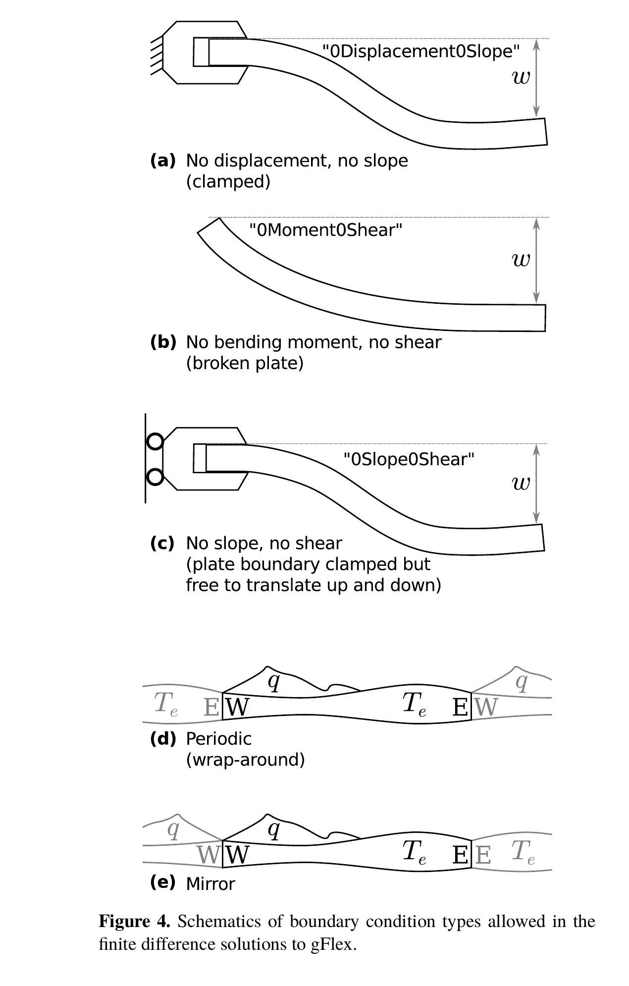
Schematics of the five finite-difference boundary condition types — Schematics of the five FD boundary condition types (a–e). Reproduced from Wickert (2016), Fig. 4; CC BY 3.0.¶

0Displacement0Slope — zero displacement and slope; plate is pinned to zero deflection at the boundary.
0Moment0Shear — zero bending moment and shear force; broken plate with a free cantilever end (Wickert, 2016, Table 1).
0Slope0Shear — zero slope and shear force; the plate is level at the boundary but free to deflect there, with no shear transmitted. Wickert (2016) calls this “free displacement of a horizontally clamped boundary.” It is superficially similar to Mirror (both enforce zero slope), but uses a different finite-difference stencil and produces noticeably different solutions; prefer Mirror for symmetry problems.
Mirror — even reflection at the boundary; model only half of a symmetric system (e.g., one flank of a mountain range or ice sheet).
Periodic — wrap-around; the domain tiles infinitely in both directions.

For SAS / SAS_NG: NoOutsideLoads (assumed if left blank).

Flexural solutions can be sensitive to boundary conditions; choose carefully and consider using pad_domain() (2-D) or pad_domain_1d() (1-D) to push boundaries away from the region of interest.

Solver

Linear system solver for FD:

direct — sparse direct solver; recommended for most grids.
iterative — lower peak memory on very large grids; slower.

ConvergenceTolerance

Relative residual tolerance passed as rtol to the LGMRES solver. Only used when Solver = iterative. Default: 1.0e-3. Decrease for higher accuracy at the cost of more iterations; the solver falls back to a direct solve if LGMRES does not converge.

Note

In-plane stresses (\(\sigma_{xx}\), \(\sigma_{yy}\), \(\sigma_{xy}\) [Pa]) cannot be set from a configuration file. They must be assigned programmatically before calling initialize():

flex.sigma_xx = 1e6   # east–west compression [Pa]
flex.sigma_yy = 0.
flex.sigma_xy = 0.

All three default to zero if not set. They are supported by FD and FFT in 2-D, and by FD and FFT in 1-D (sigma_xx only). Setting them with SAS or SAS_NG raises a warning and has no effect. See Theory for the governing equations.

`numerical2D` section¶

GridSpacing_y: Grid cell size in the y-direction [m].
BoundaryCondition_North, BoundaryCondition_South: Same options as BoundaryCondition_West / BoundaryCondition_East.
latlon: true / false. Interpret input coordinates as geographic latitude and longitude. Default: false.
PlanetaryRadius: Planetary radius [m]. Required when latlon = true. Earth: 6 371 000 m.

`verbosity` section¶

Verbose: true / false. Print progress messages during the run. Default: true.
Debug: true / false. Print internal arrays and solver diagnostics. Default: false.
Quiet: true / false. Suppress all output. Overrides Verbose and Debug. Default: false.

Complete examples¶

1-D finite-difference example (YAML)¶

# All units are SI.

mode:
  dimension: 1
  method: FD

parameter:
  YoungsModulus: 6.5e10
  PoissonsRatio: 0.25
  GravAccel: 9.8
  MantleDensity: 3300
  InfillMaterialDensity: 0

input:
  Loads: q0_sample/1D/central_block.txt
  ElasticThickness: Te_sample/1D/8km_20km_ramp.txt

output:
  DeflectionOut: ""
  Plot: combo          # overlay deflection and load (1-D only)

numerical:
  GridSpacing_x: 6000
  BoundaryCondition_West: Periodic
  BoundaryCondition_East: Periodic
  Solver: direct
  ConvergenceTolerance: 0.001

verbosity:
  Verbose: false
  Debug: false
  Quiet: false

2-D finite-difference example (YAML)¶

# All units are SI.

mode:
  dimension: 2
  method: FD
  PlateSolutionType: vWC1994   # van Wees & Cloetingh (1994); recommended

parameter:
  YoungsModulus: 6.5e10
  PoissonsRatio: 0.25
  GravAccel: 9.8
  MantleDensity: 3300
  InfillMaterialDensity: 0

input:
  Loads: q0_sample/2D/diag.txt
  ElasticThickness: Te_sample/2D/fault_24-30.txt

output:
  DeflectionOut: ""
  Plot: both

numerical:
  GridSpacing_x: 4000
  BoundaryCondition_West: 0Moment0Shear
  BoundaryCondition_East: 0Displacement0Slope
  Solver: direct
  ConvergenceTolerance: 1.0e-3

numerical2D:
  GridSpacing_y: 4000
  BoundaryCondition_North: Mirror
  BoundaryCondition_South: 0Slope0Shear

verbosity:
  Verbose: false
  Debug: false
  Quiet: false

INI format (legacy)¶

The INI format uses the same section names and parameter keys as YAML, with [section] headers and key=value pairs. Comments begin with ;. The file extension is not restricted — the absence of a .yaml / .yml suffix causes gFlex to treat the file as INI.

Equivalent 1-D example in INI:

; All units are SI.

[mode]
dimension=1
method=FD

[parameter]
YoungsModulus=6.5E10
PoissonsRatio=0.25
GravAccel=9.8
MantleDensity=3300
InfillMaterialDensity=0

[input]
Loads=q0_sample/1D/central_block.txt
ElasticThickness=Te_sample/1D/8km_20km_ramp.txt

[output]
DeflectionOut=
Plot=combo

[numerical]
GridSpacing_x=6000
BoundaryCondition_West=Periodic
BoundaryCondition_East=Periodic
Solver=direct
ConvergenceTolerance=0.001

[verbosity]
Verbose=false
Debug=false
Quiet=false

Annotated reference file (`input/input_help`)¶

The file input/input_help in the repository is an annotated INI template showing every parameter with inline comments. It is reproduced here (with corrections) for quick reference.

; input_help
; All units are SI. Not all entries are needed.
; Standard parameter values for Earth are included.

[mode]
; 1 (line) or 2 (surface) dimensions
dimension=2
; Solution method: FD (Finite Difference), SAS (Spatial domain
; analytical solutions), or SAS_NG (SAS, but on an unstructured
; grid — NG = "no grid").
; For SAS_NG, 1D data must be provided and will be returned in
; two columns: (x,q0) --> (x,w). 2D data are similar, except
; will be of the form (x,y,[q0/in or w/out]).
method=SAS
; Plate solutions can be:
;  * vWC1994 (best), or
;  * G2009 (from Govers et al., 2009; not bad, but not
;           as robust as vWC1994)
PlateSolutionType=vWC1994

[parameter]
YoungsModulus=65E9
PoissonsRatio=0.25
GravAccel=9.8
MantleDensity=3300
; This is the density of material (e.g., air, water)
; that is filling (or leaving) the hole that was
; created by flexure. If you do not have a constant
; density of infilling material, for example, at a
; subsiding shoreline, you must instead iterate.
InfillMaterialDensity=0

[input]
; space-delimited array of loads
; stresses (rho*g*h) if gridded — dx (and if applicable, dy) will be
;   applied to convert them into forces
; forces (rho*g*h*Area) if not gridded (SAS_NG)
; If the solution method is SAS_NG, this file should be of the format
; (x,[y],q0) and the code will sort it out.
Loads=q0_sample/2D/central_square_load.txt
;
; scalar value or space-delimited array of elastic thickness(es) [m]
; array required for finite difference solutions with variable Te
ElasticThickness=Te_sample/2D/10km_const.txt
;
; xw and yw are vectors of desired output points for the SAS_NG method.
; If not specified, the solution is calculated at the load points.
; Ignored for other solution methods.
xw=
yw=

[output]
; DeflectionOut is for writing an output file.
; If blank, no output file is written.
; Otherwise, a space-delimited ASCII file of deflections is written
; to this path.
DeflectionOut=tmpout.txt
;
; Acceptable inputs to "Plot" are q0 (loads), w (deflection), or both;
; any other entry results in no plotting.
; Automatically plots a 1D line or 2D surface based on "dimension".
Plot=both

[numerical]
; dx [m]
GridSpacing_x=
;
; Boundary conditions can be:
; (FD): 0Slope0Shear, 0Moment0Shear, 0Displacement0Slope, Mirror, or Periodic
; For SAS or SAS_NG, NoOutsideLoads is valid, and no entry defaults to this
BoundaryCondition_West=
BoundaryCondition_East=
;
; Solver can be direct or iterative
Solver=
; Tolerance between iterations [m]
; If you have chosen an iterative solution type, gFlex will iterate
; until the change between two subsequent iterations is below this value.
; Set as 0 if you don't want to iterate.
ConvergenceTolerance=1E-3

[numerical2D]
; dy [m]
GridSpacing_y=
;
; Boundary conditions can be:
; (FD): 0Slope0Shear, 0Moment0Shear, 0Displacement0Slope, Mirror, or Periodic
; For SAS or SAS_NG, NoOutsideLoads is valid, and no entry defaults to this
BoundaryCondition_North=
BoundaryCondition_South=
;
; Flag to enable lat/lon input (true/false). By default, this is false.
latlon=
; radius of planet [m], for lat/lon solutions
PlanetaryRadius=

[verbosity]
; true/false. Defaults to true.
Verbose=
; true/false. Defaults to false.
Debug=
; true/false -- total silence if true. Defaults to false.
Quiet=

Configuration Files¶

Parameters¶

mode section¶

parameter section¶

input section¶

output section¶

numerical section¶

numerical2D section¶

verbosity section¶